Benner’s Theory of Novice to Expert
Reply

SAMPLING:
A set of data or elements drawn from a larger population and analyzed to estimate the characteristics of that population is called sample. And the process of selecting a sample from a population is called sampling.
OR
Procedure by which some members of a given population are selected as representatives of the entire population
TYPES OF SAMPLING
There are two types of sampling
A sampling technique in which each member of the population has an equal chance of being chosen is called probability sampling.
There are four types of probability sampling
A probability sampling technique in which, each person in the population has an equal chance of being chosen for the sample and every collection of persons of the same size has an equal chance of becoming the actual sample.
A sample constructed by selecting every kth element in the sampling frame.
Number the units in the population from 1 to N decide on the n (sample size) that you want or need k = N/n = the interval size randomly select an integer between 1 to k then take every kth unit.
Is obtained by separating the population elements into non overlapping groups, called strata, and then selecting a simple random sample from each stratum.
A simple random sample in which each sampling unit is a collection or cluster, or elements. For example, an investigator wishing to study students might first sample groups or clusters of students such as classes and then select the final sample of students from among clusters. Also called area sampling.
Non-probability sampling is a sampling technique where the samples are gathered in a process that does not give all the individuals in the population equal chances of being selected.
It decreases a sample’s representativeness of a population.
Type of Non-probability sampling
Following are the common types of non-probability sampling:
The members of the population are chosen based on their relative ease of access. Suchsamples are biased because researchers may unconsciously approach some kinds of respondents and avoid others
It is the non-probability version of stratified sampling. Like stratified sampling, the researcher first identifies the stratums and their proportions as they are represented in the population. Then convenience or judgment sampling is used to select the required number of subjects from each stratum. This differs from stratified sampling, where the stratums are filled by random sampling.
It is a common non-probability method. The researcher uses his or her own judgment about which respondents to choose, and picks those who best meets the purposes of the study.
It is a special non-probability method used when the desired sample characteristic is rare. It may be extremely difficult or cost prohibitive to locate respondents in these situations. Snowball sampling relies on referrals from initial subjects to generate additional subjects. While this technique can dramatically lower search costs, it comes at the expense of introducing bias because the technique itself reduces the likelihood that the sample will represent a good cross section from the population.
INFERENTIAL STATISTICS
Statistical inference is the procedure by which we reach a conclusion about a population on the basis of the information contained in a sample drawn from that population. It consists of two techniques:
ESTIMATION OF PARAMETERS
The process of estimation entails calculating, from the data of a sample, some statistic that is offered as an approximation of the corresponding parameter of the population from which the sample was drawn.
Parameter estimation is used to estimate a single parameter, like a mean.
There are two types of estimates
POINT ESTIMATES
A point estimate is a single numerical value used to estimate the corresponding population parameter.
For example: the sample mean ‘x’ is a point estimate of the population mean μ. the sample variance S2 is a point estimate of the population variance σ2. These are point estimates — a single–valued guess of the parametric value.
A good estimator must satisfy three conditions:
CONFIDENCE INTERVAL (Interval Estimates)
An interval estimate consists of two numerical values defining a range of values that, with a specified degree of confidence, most likely includes the parameter being estimated.
Interval estimation of a parameter is more useful because it indicates a range of values within which the parameter has a specified probability of lying. With interval estimation, researchers construct a confidence interval around estimate; the upper and lower limits are called confidence limits.
Interval estimates provide a range of values for a parameter value, within which we have a stated degree of confidence that the parameter lies. A numeric range, based on a statistic and its sampling distribution that contains the population parameter of interest with a specified probability.
A confidence interval gives an estimated range of values which is likely to include an unknown population parameter, the estimated range being calculated from a given set of sample data
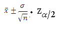
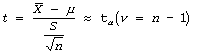
Calculating confidence interval when n ≥ 30 (Single Population Mean)
Example: A random sample of size 64 with mean 25 & Standard Deviation 4 is taken from a normal population. Construct 95 % confidence interval
We use following formula to solve Confidence Interval when n ≥ 30
Data
= 4
n = 64
![]()
![]() 25 4/
25 4/![]() . x 1.96
. x 1.96
![]() 25 4/8 x 1.96
25 4/8 x 1.96
![]() 25 0.5 x 1.96
25 0.5 x 1.96
![]() 25 0.98
25 0.98
25 – 0.98 ≤ µ ≤ 25 + 0.98
24.02≤ µ ≤ 25.98
We are 95% confident that population mean (µ) will have value between 24.02 & 25.98
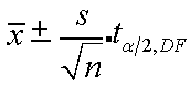
Calculating confidence interval when n < 30 (Single Population Mean)
Example: A random sample of size 9 with mean 25 & Standard Deviation 4 is taken from a normal population. Construct 95 % confidence interval
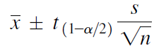
We use following formula to solve Confidence Interval when n < 30
(OR)
Data
S = 4
n = 9
α/2 = 0.025
df = n – 1 (9 -1 = 8)
tα/2,df = 2.306
25 ± 4/√9 x 2.306
25 ± 4/3 x 2.306
25 ± 1.33 x 2.306
25 ± 3.07
25 – 3.07 ≤ µ ≤ 25 + 3.07
21.93 ≤ µ ≤ 28.07
We are 95% confident that population mean (µ) will have value between 21.93 & 28.07
Hypothesis:
A hypothesis may be defined simply as a statement about one or more populations. It is frequently concerned with the parameters of the populations about which the statement is made.
Types of Hypotheses
Researchers are concerned with two types of hypotheses
The research hypothesis is the conjecture or supposition that motivates the research. It may be the result of years of observation on the part of the researcher.
Statistical hypotheses are hypotheses that are stated in such a way that they may be evaluated by appropriate statistical techniques.
Types of statistical Hypothesis
There are two statistical hypotheses involved in hypothesis testing, and these should be stated explicitly.
The null hypothesis is the hypothesis to be tested. It is designated by the symbol Ho. The null hypothesis is sometimes referred to as a hypothesis of no difference, since it is a statement of agreement with (or no difference from) conditions presumed to be true in the population of interest.
In general, the null hypothesis is set up for the express purpose of being discredited. Consequently, the complement of the conclusion that the researcher is seeking to reach becomes the statement of the null hypothesis. In the testing process the null hypothesis either is rejected or is not rejected. If the null hypothesis is not rejected, we will say that the data on which the test is based do not provide sufficient evidence to cause rejection. If the testing procedure leads to rejection, we will say that the data at hand are not compatible with the null hypothesis, but are supportive of some other hypothesis.
The alternative hypothesis is a statement of what we will believe is true if our sample data cause us to reject the null hypothesis. Usually the alternative hypothesis and the research hypothesis are the same, and in fact the two terms are used interchangeably. We shall designate the alternative hypothesis by the symbol HA orH1.
LEVEL OF SIGNIFICANCE
The level of significance is a probability and, in fact, is the probability of rejecting a true null hypothesis. The level of significance specifies the area under the curve of the distribution of the test statistic that is above the values on the horizontal axis constituting the rejection region. It is denoted by ‘α’.
Types of Error
In the context of testing of hypotheses, there are basically two types of errors:
Type I Error
Type II Error
In the tabular form two errors can be presented as follows:
| Null hypothesis (H0) is true | Null hypothesis (H0) is false | |
| Reject null hypothesis | Type I error False positive |
Correct outcome True positive |
| Fail to reject null hypothesis | Correct outcome True negative |
Type II error False negative |
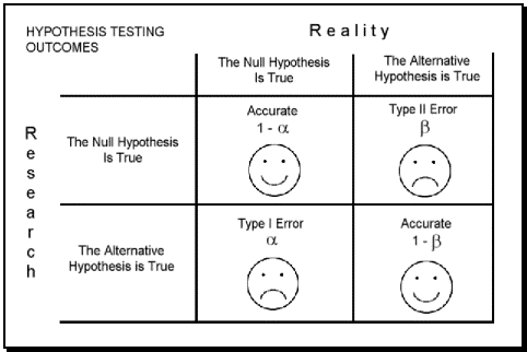
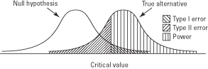 Graphical depiction of the relation between Type I and Type II errors
What are the differences between Type 1 errors and Type 2 errors?
| Type 1 Error | Type 2 Error |
|
|
Reducing Type I Errors
Reducing Type II Errors
Power of Test:
Statistical power is defined as the probability of rejecting the null hypothesis while the alternative hypothesis is true.
Power = P(reject H0 | H1 is true)
= 1 – P(type II error)
= 1 – β
That is, the power of a hypothesis test is the probability that it will reject when it’s supposed to.
Distribution under H0
Distribution under H1
| Power |
Factors that affect statistical power include
Application:
In research, statistical power is generally calculated for two purposes.
Relation with sample size:
Statistical power is positively correlated with the sample size, which means that given the level of the other factors, a larger sample size gives greater power. However, researchers are also faced with the decision to make a difference between statistical difference and scientific difference. Although a larger sample size enables researchers to find smaller difference statistically significant, that difference may not be large enough be scientifically meaningful. Therefore, this would be recommended that researcher have an idea of what they would expect to be a scientifically meaningful difference before doing a power analysis to determine the actual sample size needed.
HYPOTHESIS TESTING
Statistical hypothesis testing provides objective criteria for deciding whether hypotheses are supported by empirical evidence.
The purpose of hypothesis testing is to aid the clinician, researcher, or administrator in reaching a conclusion concerning a population by examining a sample from that population.
STEPS IN STATISTICAL HYPOTHESIS TESTING
Step # 01: State the Null hypothesis and Alternative hypothesis.
The alternative hypothesis represents what the researcher is trying to prove. The null hypothesis represents the negation of what the researcher is trying to prove.
Step # 02: State the significance level, α (0.01, 0.05, or 0.1), for the test
The significance level is the probability of making a Type I error. A Type I Error is a decision in favor of the alternative hypothesis when, in fact, the null hypothesis is true.
Type II Error is a decision to fail to reject the null hypothesis when, in fact, the null hypothesis is false.
Step # 03: State the test statistic that will be used to conduct the hypothesis test
The appropriate test statistic for different kinds of hypothesis tests (i.e. t-test, z-test, ANOVA, Chi-square etc.) are stated in this step
Step # 04: Computation/ calculation of test statistic
Different kinds of hypothesis tests (i.e. t-test, z-test, ANOVA, Chi-square etc.) are computed in this step.
Step # 05: Find Critical Value or Rejection (critical) Region of the test
Use the value of α (0.01, 0.05, or 0.1) from Step # 02 and the distribution of the test statistics from Step # 03.
Step # 06: Conclusion (Making statistical decision and interpretation of results)
If calculated value of test statistics falls in the rejection (critical) region, the null hypothesis is rejected, while, if calculated value of test statistics falls in the acceptance (noncritical) region, the null hypothesis is not rejected i.e. it is accepted.
Note: In case if we conclude on the basis of p-value then we compare calculated p-value to the chosen level of significance. If p-value is less than α, then the null hypothesis will be rejected and alternative will be affirmed. If p-value is greater than α, then the null hypothesis will not be rejected
If the decision is to reject, the statement of the conclusion should read as follows: “we reject at the _______ level of significance. There is sufficient evidence to conclude that (statement of alternative hypothesis.)”
If the decision is to fail to reject, the statement of the conclusion should read as follows: “we fail to reject at the _______ level of significance. There is no sufficient evidence to conclude that (statement of alternative hypothesis.)”
Rules for Stating Statistical Hypotheses
When hypotheses are stated, an indication of equality (either = ,≤ or ≥ ) must appear in the null hypothesis.
Example:
We want to answer the question: Can we conclude that a certain population mean is not 50? The null hypothesis is
Ho : µ = 50
And the alternative is
HA : µ ≠ 50
Suppose we want to know if we can conclude that the population mean is greater than
50. Our hypotheses are
Ho: µ ≤ 50
HA: µ >
If we want to know if we can conclude that the population mean is less than 50, the hypotheses are
Ho : µ ≥ 50
HA: µ < 50
We may state the following rules of thumb for deciding what statement goes in the null hypothesis and what statement goes in the alternative hypothesis:
T- TEST
T-test is used to test hypotheses about μ when the population standard deviation is unknown and Sample size can be small (n<30).
The distribution is symmetrical, bell-shaped, and similar to the normal but more spread out.
Calculating one sample t-test
Example: A random sample of size 16 with mean 25 and Standard Deviation 5 is taken from a normal population Test at 5% LOS that; : µ= 22
: µ≠22
SOLUTION
Step # 01: State the Null hypothesis and Alternative hypothesis.
: µ= 22
: µ≠22
Step # 02: State the significance level
α = 0.05 or 5% Level of Significance
 Step # 03: State the test statistic (n<30)
t-test statistic
Step # 04: Computation/ calculation of test statistic


Data
µ = 22
S = 5
n = 16

![]()
t calculated = 2.4
Step # 05: Find Critical Value or Rejection (critical) Region
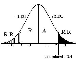
For critical value we find and on the basis of its answer we see critical value from t-distribution table.
![]()
Critical value = α/2(v = 16-1)
= 0.05/2(v = 15)
= (0.025, 15)
t tabulated = ± 2.131
t calculated = 2.4
Step # 06: Conclusion: Since t calculated = 2.4 falls in the region of rejection therefore we reject at the 5% level of significance. There is sufficient evidence to conclude that Population mean is not equal to 22.
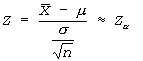
Z- TEST
Calculating one sample z-test
Example: A random sample of size 49 with mean 32 is taken from a normal population whose standard deviation is 4. Test at 5% LOS that : µ= 25
: µ≠25
SOLUTION
Step # 01: : µ= 25
: µ≠25
Step # 02: α = 0.05
Step # 03:Since (n<30), we apply z-test statistic
Step # 04: Calculation of test statistic


Data
µ = 25
= 4
n = 49


Zcalculated = 12.28
Step # 05: Find Critical Value or Rejection (critical) Region
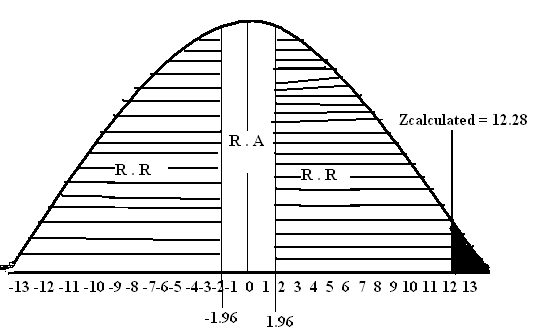
Critical Value (5%) (2-tail) = ±1.96
Zcalculated = 12.28
Step # 06: Conclusion: Since Zcalculated = 12.28 falls in the region of rejection therefore we reject at the 5% level of significance. There is sufficient evidence to conclude that Population mean is not equal to 25.
CHI-SQUARE
A statistic which measures the discrepancy (difference) between KObserved Frequencies fo1, fo2… fok and the corresponding ExpectedFrequencies fe1, fe2……. fek
The chi-square is useful in making statistical inferences about categorical data in whichthe categories are two and above.
Characteristics
Calculating Chi-Square
Example 1: census of U.S. determine four categories of doctors practiced in different areas as
| Specialty | % | Probability |
| General Practice | 18% | 0.18 |
| Medical | 33.9 % | 0.339 |
| Surgical | 27 % | 0.27 |
| Others | 21.1 % | 0.211 |
| Total | 100 % | 1.000 |
A searcher conduct a test after 5 years to check this data for changes and select 500 doctors and asked their speciality. The result were:
| Specialty | frequency |
| General Practice | 80 |
| Medical | 162 |
| Surgical | 156 |
| Others | 102 |
| Total | 500 |
Hypothesis testing:
Step 01”
Null Hypothesis (Ho):
There is no difference in specialty distribution (or) the current specialty distribution of US physician is same as declared in the census.
Alternative Hypothesis (HA):
There is difference in specialty distribution of US doctors. (or) the current specialty distribution of US physician is different as declared in the census.
Step 02: Level of Significance
α = 0.05
Step # 03:Chi-squire Test Statistic
Step # 04:
Statistical Calculation
fe (80) = 18 % x 500 = 90
fe (162) = 33.9 % x 500 = 169.5
fe (156) = 27 % x 500 = 135
fe (102) = 21.1 % x 500 = 105.5
| S # (n) | Specialty | fo | fe | (fo – fe) | (fo – fe) 2 | (fo – fe) 2 / fe |
| 1 | General Practice | 80 | 90 | -10 | 100 | 1.11 |
| 2 | Medical | 162 | 169.5 | -7.5 | 56.25 | 0.33 |
| 3 | Surgical | 156 | 135 | 21 | 441 | 3.26 |
| 4 | Others | 102 | 105.5 | -3.5 | 12.25 | 0.116 |
| 4.816 | ||||||
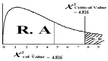 χ2cal= = 4.816
Step # 05:
Find critical region using X2– chi-squire distribution table
χ2 = χ2 = χ2 = 7.815
tab (α,d.f) (0.05,3)
(d.f = n – 1)
Step # 06:
Conclusion: Since χ2cal value lies in the region of acceptance therefore we accept the HO and reject HA. There is no difference in specialty distribution among U.S. doctors.
Example2: A sample of 150 chronic Carriers of certain antigen and a sample of 500 Non-carriers revealed the following blood group distributions. Can one conclude from these data that the two population from which samples were drawn differ with respect to blood group distribution? Let α = 0.05.
| Blood Group | Carriers | Non-carriers | Total |
| O | 72 | 230 | 302 |
| A | 54 | 192 | 246 |
| B | 16 | 63 | 79 |
| AB | 8 | 15 | 23 |
| Total | 150 | 500 | 650 |
Hypothesis Testing
Step # 01: HO: There is no association b/w Antigen and Blood Group
HA: There is some association b/w Antigen and Blood Group
Step # 02:α = 0.05
Step # 03:Chi-squire Test Statistic
Step # 04:
Calculation
fe (72) = 302*150/650 = 70
fe (230) = 302*500/ 650 = 232
fe (54) = 246*150/650 = 57
fe (192) = 246*500/650 = 189
fe (16) = 79*150/650 = 18
fe (63) = 79*500/650 = 61
fe (8) = 23*150/650 = 05
fe (15) = 23*500/650 = 18
| fo | fe | (fo – fe) | (fo – fe) 2 | (fo – fe) 2 / fe |
| 72 | 70 | 2 | 4 | 0.0571 |
| 230 | 232 | -2 | 4 | 0.0172 |
| 54 | 57 | -3 | 9 | 0.1578 |
| 192 | 189 | 3 | 9 | 0.0476 |
| 16 | 18 | -2 | 4 | 0.2222 |
| 63 | 61 | 2 | 4 | 0.0655 |
| 8 | 5 | 3 | 9 | 1.8 |
| 15 | 18 | -3 | 9 | 0.5 |
| 2.8674 | ||||
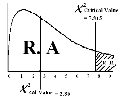 X2 = = 2.8674
X2cal = 2.8674
Step # 05:
Find critical region using X2– chi-squire distribution table
X2 = (α, d.f) = (0.05, 3) = 7.815
Step # 06:
Conclusion: Since X2cal value lies in the region of acceptance therefore we accept the HO andreject HA. Means There is no association b/w Antigen and Blood Group
WHAT IS TEST OF SIGNIFICANCE? WHY IT IS NECESSARY? MENTION NAMES OF IMPORTANT TESTS.
1. Test of significance
A procedure used to establish the validity of a claim by determining whether or not the test statistic falls in the critical region. If it does, the results are referred to as significant. This test is sometimes called the hypothesis test.
The methods of inference used to support or reject claims based on sample data are known as tests of significance.
Why it is necessary
A significance test is performed;
Types of test of significance
P –Value:
A p-value is the probability that the computed value of a test statistic is at least as extreme as a specified value of the test statistic when the null hypothesis is true. Thus, the p value is the smallest value of for which we can reject a null hypothesis.
Simply the p value for a test may be defined also as the smallest value of α for which the null hypothesis can be rejected.
The p value is a number that tells us how unusual our sample results are, given that the null hypothesis is true. A p value indicating that the sample results are not likely to have occurred, if the null hypothesis is true, provides justification for doubting the truth of the null hypothesis.
Test Decisions with p-value
The decision about whether there is enough evidence to reject the null hypothesis can be made by comparing the p-values to the value of α, the level of significance of the test.
A general rule worth remembering is:
| If p-value ≤ α reject the null hypothesis |
| If p-value ≥ α fail to reject the null hypothesis |
Observational Study:
An observational study is a scientific investigation in which neither the subjects under study nor any of the variables of interest are manipulated in any way.
An observational study, in other words, may be defined simply as an investigation that is not an experiment. The simplest form of observational study is one in which there are only two variables of interest. One of the variables is called the risk factor, or independent variable, and the other variable is referred to as the outcome, or dependent variable.
Risk Factor:
The term risk factor is used to designate a variable that is thought to be related to some outcome variable. The risk factor may be a suspected cause of some specific state of the outcome variable.
Types of Observational Studies
There are two basic types of observational studies, prospective studies and retrospective studies.
Prospective Study:
A prospective study is an observational study in which two random samples of subjects are selected. One sample consists of subjects who possess the risk factor, and the other sample consists of subjects who do not possess the risk factor. The subjects are followed into the future (that is, they are followed prospectively), and a record is kept on the number of subjects in each sample who, at some point in time, are classifiable into each of the categories of the outcome variable.
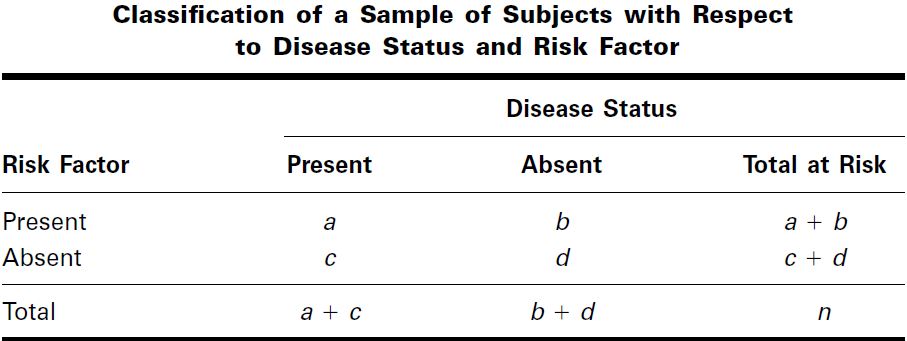
The data resulting from a prospective study involving two dichotomous variables can be displayed in a 2 x 2 contingency table that usually provides information regarding the number of subjects with and without the risk factor and the number who did and did not
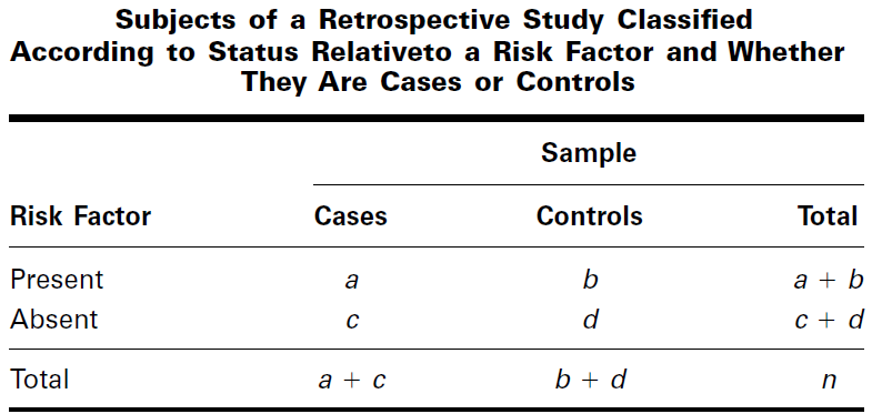
Retrospective Study:
A retrospective study is the reverse of a prospective study. The samples are selected from those falling into the categories of the outcome variable. The investigator then looks back (that is, takes a retrospective look) at the subjects and determines which ones have (or had) and which ones do not have (or did not have) the risk factor.
From the data of a retrospective study we may construct a contingency table
Relative Risk:
Relative risk is the ratio of the risk of developing a disease among subjects with the risk factor to the risk of developing the disease among subjects without the risk factor.
We represent the relative risk from a prospective study symbolically as
We may construct a confidence interval for RR
100 (1 – α)%CI=
Where zα is the two-sided z value corresponding to the chosen confidence coefficient and X2is computed by Equation
Interpretation of RR
EXAMPLE
In a prospective study of pregnant women, Magann et al. (A-16) collected extensive information on exercise level of low-risk pregnant working women. A group of 217 women did no voluntary or mandatory exercise during the pregnancy, while a group of
238 women exercised extensively. One outcome variable of interest was experiencing preterm labor. The results are summarized in Table
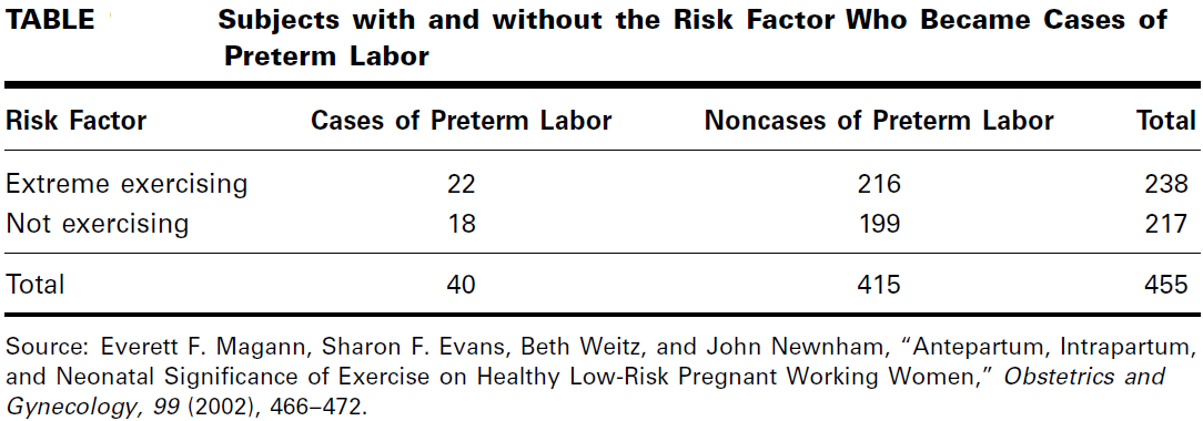
Estimate the relative risk of preterm labor when pregnant women exercise extensively.
Solution:
By Equation
These data indicate that the risk of experiencing preterm labor when a woman exercises heavily is 1.1 times as great as it is among women who do not exercise at all.
Confidence Interval for RR
We compute the 95 percent confidence interval for RR as follows.
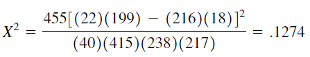
The lower and upper confidence limits are, respectively
= 0.65 and = 1.86
Conclusion:
Since the interval includes 1, we conclude, at the .05 level of significance, that the population risk may be 1. In other words, we conclude that, in the population, there may not be an increased risk of experiencing preterm labor when a pregnant woman exercises extensively.
Odds Ratio
An odds ratio (OR) is a measure of association between an exposure and an outcome. The OR represents the odds that an outcome will occur given a particular exposure, compared to the odds of the outcome occurring in the absence of that exposure.
It is the appropriate measure for comparing cases and controls in a retrospective study.
Odds:
The odds for success are the ratio of the probability of success to the probability of failure.
Two odds that we can calculate from data displayed as in contingency Table of retrospective study
The estimate of the population odds ratio is
We may construct a confidence interval for OR by the following method:
100 (1 – α) %CI=
Where is the two-sided z value corresponding to the chosen confidence coefficient and X2 is computed by Equation
Interpretation of the Odds Ratio:
In the case of a rare disease, the population odds ratio provides a good approximation to the population relative risk. Consequently, the sample odds ratio, being an estimate of the population odds ratio, provides an indirect estimate of the population relative risk in the case of a rare disease.
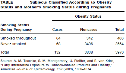
EXAMPLE
Toschke et al. (A-17) collected data on obesity status of children ages 5–6 years and the smoking status of the mother during the pregnancy. Table below shows 3970 subjects classified as cases or noncases of obesity and also classified according to smoking status of the mother during pregnancy (the risk factor).
We wish to compare the odds of obesity at ages 5–6 among those whose mother smoked throughout the pregnancy with the odds of obesity at age 5–6 among those whose mother did not smoke during pregnancy.
Solution
By formula:
We see that obese children (cases) are 9.62 times as likely as nonobese children (noncases) to have had a mother who smoked throughout the pregnancy.
We compute the 95 percent confidence interval for OR as follows.
The lower and upper confidence limits for the population OR, respectively, are
= 7.12 and = = 13.00
We conclude with 95 percent confidence that the population OR is somewhere between
7.12 And 13.00. Because the interval does not include 1, we conclude that, in the population, obese children (cases) are more likely than nonobese children (noncases) to have had a mother who smoked throughout the pregnancy.
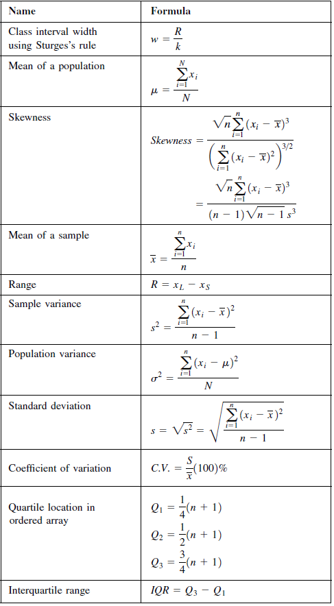
Measures of Dispersion
This term is used commonly to mean scatter, Deviation, Fluctuation, Spread or variability of data.
The degree to which the individual values of the variate scatter away from the average or the central value, is called a dispersion.
Types of Measures of Dispersions:
![]()
Absolute Measures
Relative Measure
The Range:
1. The range is the simplest measure of dispersion. It is defined as the difference between the largest value and the smallest value in the data:
![]()
2. For grouped data, the range is defined as the difference between the upper class boundary (UCB) of the highest class and the lower class boundary (LCB) of the lowest class.
MERITS OF RANGE:-
DEMERITS OF RANGE:-
Quartile Deviation (QD):
1. It is also known as the Semi-Interquartile Range. The range is a poor measure of dispersion where extremely large values are present. The quartile deviation is defined half of the difference between the third and the first quartiles:
QD = Q3 – Q1/2
Inter-Quartile Range
The difference between third and first quartiles is called the ‘Inter-Quartile Range’.
IQR = Q3 – Q1
Mean Deviation (MD):
1. The MD is defined as the average of the deviations of the values from an average:
![]()
It is also known as Mean Absolute Deviation.
2. MD from median is expressed as follows:
![]()
3. for grouped data:
The Variance:
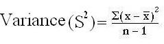 Formula
OR S2 =
Calculating variance: Heart rate of certain patient is 80, 84, 80, 72, 76, 88, 84, 80, 78, & 78. Calculate variance for this data.
Solution:
Step 1:
Find mean of this data
![]()
= 800/10 Mean = 80
Step 2:
Draw two Columns respectively ‘X’ and deviation about mean (X-
![]()
). In column ‘X’ put all values of X and in (X-
![]()
) subtract each ‘X’ value with
![]()
.
Step 3:
Draw another Column of (X-
![]()
) 2, in which put square of deviation about mean.
| X |
(X- ) Deviation about mean |
(X- )2 Square of Deviation about mean |
|
80
84 80 72 76 88 84 80 78 78 |
80 – 80 = 0
84 – 80 = 4 80 – 80 = 0 72 – 80 = -8 76 – 80 = -4 88 – 80 = 8 84 – 80 = 4 80 – 80 = 0 78 – 80 = -2 78 – 80 = -2 |
0 x 0 = 00
4 x 4 = 16 0 x 0 = 00 -8 x -8 = 64 -4 x -4 = 16 8 x 8 = 64 4 x 4 = 16 0 x 0 = 00 -2 x -2 = 04 -2 x -2 = 04 |
|
∑X = 800
|
∑(X- ) = 0 Summation of Deviation about mean is always zero |
∑(X- )2 = 184 Summation of Square of Deviation about mean |
Step 4
Apply formula and put following values
∑(X-
![]()
) 2= 184
n = 10

Variance = 184/ 10-1 = 184/9
Variance = 20.44
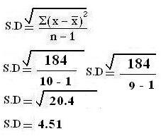
Standard Deviation
 Formula:
OR S =
Calculating Standard Deviation (we use same example): Heart rate of certain patient is 80, 84, 80, 72, 76, 88, 84, 80, 78, & 78. Calculate standard deviation for this data.
SOLUTION:
Step 1: Find mean of this data
![]()
= 800/10 Mean = 80
Step 2:
Draw two Columns respectively ‘X’ and deviation about mean (X-). In column ‘X’ put all values of X and in (X-) subtract each ‘X’ value with.
Step 3:
Draw another Column of (X-![]()
) 2, in which put square of deviation about mean.
| X |
(X- ) Deviation about mean |
(X- )2 Square of Deviation about mean |
|
80
84 80 72 76 88 84 80 78 78 |
80 – 80 = 0
84 – 80 = 4 80 – 80 = 0 72 – 80 = -8 76 – 80 = -4 88 – 80 = 8 84 – 80 = 4 80 – 80 = 0 78 – 80 = -2 78 – 80 = -2 |
0 x 0 = 00
4 x 4 = 16 0 x 0 = 00 -8 x -8 = 64 -4 x -4 = 16 8 x 8 = 64 4 x 4 = 16 0 x 0 = 00 -2 x -2 = 04 -2 x -2 = 04 |
|
∑X = 800
|
∑(X- ) = 0 Summation of Deviation about mean is always zero |
∑(X- )2 = 184 Summation of Square of Deviation about mean |
Step 4
Apply formula and put following values
∑(X-
![]()
)2 = 184
n = 10
MERITS AND DEMERITS OF STD. DEVIATION
DEMERITS-
Relative measure of dispersion:
(a) Coefficient of Variation,
(b) Coefficient of Dispersion,
(c) Quartile Coefficient of Dispersion, and
(d) Mean Coefficient of Dispersion.
Coefficient of Variation (CV):
1. Coefficient of variation was introduced by Karl Pearson. The CV expresses the SD as a percentage in terms of AM:
![]()
—————- For sample data
![]()
————— For population data
Coefficient of Dispersion (CD):
If Xm and Xn are respectively the maximum and the minimum values in a set of data, then the coefficient of dispersion is defined as:
![]()
Coefficient of Quartile Deviation (CQD):
1. If Q1 and Q3 are given for a set of data, then (Q1 + Q3)/2 is a measure of central tendency or average of data. Then the measure of relative dispersion for quartile deviation is expressed as follows:
![]()
CQD may also be expressed in percentage.
Mean Coefficient of Dispersion (CMD):
The relative measure for mean deviation is ‘mean coefficient of dispersion’ or ‘coefficient of mean deviation’:
![]()
——————– for arithmetic mean
![]()
——————– for median
Percentiles and Quartiles
The mean and median are special cases of a family of parameters known as location parameters. These descriptive measures are called location parameters because they can be used to designate certain positions on the horizontal axis when the distribution of a variable is graphed.
Percentile:
Percentiles corresponding to a given data value: The percentile in a set corresponding to a specific data value is obtained by using the following formula
Number of values below X + 0.5
Percentile = ——————————————–
Number of total values in data set
Example: Calculate percentile for value 12 from the following data
13 11 10 13 11 10 8 12 9 9 8 9
Solution:
Step # 01: Arrange data values in ascending order from smallest to largest
| S. No | 1 | 2 | 3 | 4 | 5 | 6 | 7 | 8 | 9 | 10 | 11 | 12 |
| Observations or values | 8 | 8 | 9 | 9 | 9 | 10 | 10 | 11 | 11 | 12 | 13 | 13 |
Step # 02: The number of values below 12 is 9 and total number in the data set is 12
Step # 03: Use percentile formula
9 + 0.5
Percentile for 12 = ——— x 100 = 79.17%
12
It means the value of 12 corresponds to 79th percentile
Example2: Find out 25th percentile for the following data
6 12 18 12 13 8 13 11
10 16 13 11 10 10 2 14
SOLUTION
Step # 01: Arrange data values in ascending order from smallest to largest
| S. No | 1 | 2 | 3 | 4 | 5 | 6 | 7 | 8 | 9 | 10 | 11 | 12 | 13 | 14 | 15 | 16 |
| Observations or values | 2 | 6 | 8 | 10 | 10 | 10 | 11 | 11 | 12 | 12 | 13 | 13 | 13 | 14 | 16 | 18 |
Step # 2 Calculate the position of percentile (n x k/ 100). Here n = No: of observation = 16 and k (percentile) = 25
16 x 25 16 x 1
Therefore Percentile = ———- = ——— = 4
100 4
Therefore, 25th percentile will be the average of values located at the 4th and 5th position in the ordered set. Here values for 4th and 5th correspond to the value of 10 each.
(10 + 10)
Thus, P25 (=Pk) = ————– = 10
2
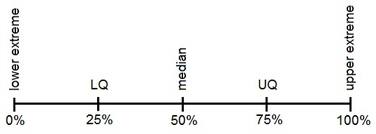
Quartiles
These are measures of position which divide the data into four equal parts when the data is arranged in ascending or descending order. The quartiles are denoted by Q.
| Quartiles | Formula for Ungrouped Data | Formula for Grouped Data |
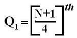
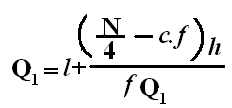
| Q1 = First Quartile below which first 25% of the observations are present |
 |
 |
|
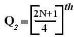
Q2 = Second Quartile below which first 50% of the observations are present.
It can easily be located as the median value. |
 |
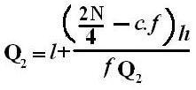 |
| Q3 = Third Quartile below which first 75% of the observations are present |
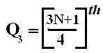 |
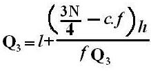 |
Symbol Key:
