Statistical inference is the procedure by which we reach a conclusion about a population on the basis of the information contained in a sample drawn from that population. It consists of two techniques:
- Estimation of parameters
- Hypothesis testing
ESTIMATION OF PARAMETERS
The process of estimation entails calculating, from the data of a sample, some statistic that is offered as an approximation of the corresponding parameter of the population from which the sample was drawn.
Parameter estimation is used to estimate a single parameter, like a mean.
There are two types of estimates
- Point Estimates
- Interval Estimates (Confidence Interval).
POINT ESTIMATES
A point estimate is a single numerical value used to estimate the corresponding population parameter.
For example: the sample mean ‘x’ is a point estimate of the population mean μ. the sample variance S2 is a point estimate of the population variance σ2. These are point estimates — a single–valued guess of the parametric value.
A good estimator must satisfy three conditions:
- Unbiased: The expected value of the estimator must be equal to the mean of the parameter
- Consistent: The value of the estimator approaches the value of the parameter as the sample size increases
- Relatively Efficient: The estimator has the smallest variance of all estimators which could be used
CONFIDENCE INTERVAL (Interval Estimates)
An interval estimate consists of two numerical values defining a range of values that, with a specified degree of confidence, most likely includes the parameter being estimated.
Interval estimation of a parameter is more useful because it indicates a range of values within which the parameter has a specified probability of lying. With interval estimation, researchers construct a confidence interval around estimate; the upper and lower limits are called confidence limits.
Interval estimates provide a range of values for a parameter value, within which we have a stated degree of confidence that the parameter lies. A numeric range, based on a statistic and its sampling distribution that contains the population parameter of interest with a specified probability.
A confidence interval gives an estimated range of values which is likely to include an unknown population parameter, the estimated range being calculated from a given set of sample data
Calculating confidence interval when n ≥ 30 (Single Population Mean)
Example: A random sample of size 64 with mean 25 & Standard Deviation 4 is taken from a normal population. Construct 95 % confidence interval
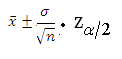
We use following formula to solve Confidence Interval when n ≥ 30
Data
= 4
n = 64
 25 4/
25 4/ . x 1.96
 25 4/8 x 1.96
 25 0.5 x 1.96
 25 0.98
25 – 0.98 ≤ µ ≤ 25 + 0.98
24.02≤ µ ≤ 25.98
We are 95% confident that population mean (µ) will have value between 24.02 & 25.98
Calculating confidence interval when n < 30 (Single Population Mean)
Example: A random sample of size 9 with mean 25 & Standard Deviation 4 is taken from a normal population. Construct 95 % confidence interval
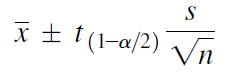 We use following formula to solve Confidence Interval when n < 30
(OR)
Data
S = 4
n = 9
α/2 = 0.025
df = n – 1 (9 -1 = 8)
tα/2,df = 2.306
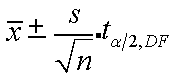
25 ± 4/√9 x 2.306
25 ± 4/3 x 2.306
25 ± 1.33 x 2.306
25 ± 3.07
25 – 3.07 ≤ µ ≤ 25 + 3.07
21.93 ≤ µ ≤ 28.07
We are 95% confident that population mean (µ) will have value between 21.93 & 28.07
Hypothesis:
A hypothesis may be defined simply as a statement about one or more populations. It is frequently concerned with the parameters of the populations about which the statement is made.
Types of Hypotheses
Researchers are concerned with two types of hypotheses
- Research hypotheses
The research hypothesis is the conjecture or supposition that motivates the research. It may be the result of years of observation on the part of the researcher.
- Statistical hypotheses
Statistical hypotheses are hypotheses that are stated in such a way that they may be evaluated by appropriate statistical techniques.
Types of statistical Hypothesis
There are two statistical hypotheses involved in hypothesis testing, and these should be stated explicitly.
- Null Hypothesis:
The null hypothesis is the hypothesis to be tested. It is designated by the symbol Ho. The null hypothesis is sometimes referred to as a hypothesis of no difference, since it is a statement of agreement with (or no difference from) conditions presumed to be true in the population of interest.
In general, the null hypothesis is set up for the express purpose of being discredited. Consequently, the complement of the conclusion that the researcher is seeking to reach becomes the statement of the null hypothesis. In the testing process the null hypothesis either is rejected or is not rejected. If the null hypothesis is not rejected, we will say that the data on which the test is based do not provide sufficient evidence to cause rejection. If the testing procedure leads to rejection, we will say that the data at hand are not compatible with the null hypothesis, but are supportive of some other hypothesis.
- Alternative Hypothesis
The alternative hypothesis is a statement of what we will believe is true if our sample data cause us to reject the null hypothesis. Usually the alternative hypothesis and the research hypothesis are the same, and in fact the two terms are used interchangeably. We shall designate the alternative hypothesis by the symbol HA orH1.
LEVEL OF SIGNIFICANCE
The level of significance is a probability and, in fact, is the probability of rejecting a true null hypothesis. The level of significance specifies the area under the curve of the distribution of the test statistic that is above the values on the horizontal axis constituting the rejection region. It is denoted by ‘α’.
Types of Error
In the context of testing of hypotheses, there are basically two types of errors:
- TYPE I Error
- TYPE II Error
Type I Error
- A type I error, also known as an error of the first kind, occurs when the null hypothesis (H0) is true, but is rejected.
- A type I error may be compared with a so called false positive.
- The rate of the type I error is called the size of the test and denoted by the Greek letter α (alpha).
- It usually equals the significance level of a test.
- If type I error is fixed at 5 %, it means that there are about 5 chances in 100 that we will reject H0 when H0 is true.
Type II Error
- Type II error, also known as an error of the second kind, occurs when the null hypothesis is false, but erroneously fails to be rejected.
- Type II error means accepting the hypothesis which should have been rejected.
- A Type II error is committed when we fail to believe a truth.
- A type II error occurs when one rejects the alternative hypothesis (fails to reject the null hypothesis) when the alternative hypothesis is true.
- The rate of the type II error is denoted by the Greek letter β (beta) and related to the power of a test (which equals 1-β ).
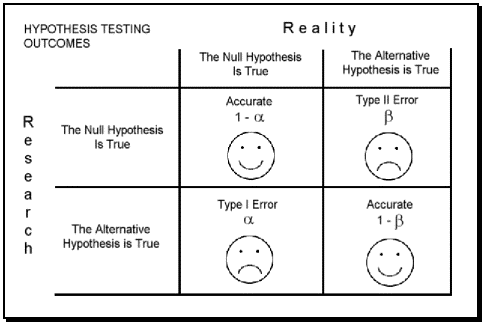
In the tabular form two errors can be presented as follows:
|
Null hypothesis (H0) is true |
Null hypothesis (H0) is false |
| Reject null hypothesis |
Type I error
False positive |
Correct outcome
True positive |
| Fail to reject null hypothesis |
Correct outcome
True negative |
Type II error
False negative |
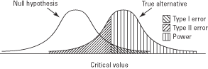 Graphical depiction of the relation between Type I and Type II errors
What are the differences between Type 1 errors and Type 2 errors?
| Type 1 Error |
Type 2 Error |
- A type 1 error is when a statistic calls for the rejection of a null hypothesis which is factually true.
- We may reject H0 when H0 is true is known as Type I error .
- A type 1 error is called a false positive.
- It denoted by the Greek letter α (alpha).
- Null hypothesis and type I error
|
- A type 2 error is when a statistic does not give enough evidence to reject a null hypothesis even when the null hypothesis should factually be rejected.
- We may accept H0 when infect H0 is not true is known as Type II Error.
- A type 2 error is a false negative.
- It denoted by “β” (beta)
- Alternative hypothesis and type II error.
|
Reducing Type I Errors
- Prescriptive testing is used to increase the level of confidence, which in turn reduces Type I errors. The chances of making a Type I error are reduced by increasing the level of confidence.
Reducing Type II Errors
- Descriptive testing is used to better describe the test condition and acceptance criteria, which in turn reduces type ii errors. This increases the number of times we reject the null hypothesis – with a resulting increase in the number of type I errors (rejecting H0 when it was really true and should not have been rejected).
- Therefore, reducing one type of error comes at the expense of increasing the other type of error! The same means cannot reduce both types of errors simultaneously.
Power of Test:
Statistical power is defined as the probability of rejecting the null hypothesis while the alternative hypothesis is true.
Power = P(reject H0 | H1 is true)
= 1 – P(type II error)
= 1 – β
That is, the power of a hypothesis test is the probability that it will reject when it’s supposed to.
Distribution under H0
Distribution under H1
Factors that affect statistical power include
- The sample size
- The specification of the parameter(s) in the null and alternative hypothesis, i.e. how far they are from each other, the precision or uncertainty the researcher allows for the study (generally the confidence or significance level)
- The distribution of the parameter to be estimated. For example, if a researcher knows that the statistics in the study follow a Z or standard normal distribution, there are two parameters that he/she needs to estimate, the population mean (μ) and the population variance (σ2). Most of the time, the researcher know one of the parameters and need to estimate the other. If that is not the case, some other distribution may be used, for example, if the researcher does not know the population variance, he/she can estimate it using the sample variance and that ends up with using a T distribution.
Application:
In research, statistical power is generally calculated for two purposes.
- It can be calculated before data collection based on information from previous research to decide the sample size needed for the study.
- It can also be calculated after data analysis. It usually happens when the result turns out to be non-significant. In this case, statistical power is calculated to verify whether the non-significant result is due to really no relation in the sample or due to a lack of statistical power.
Relation with sample size:
Statistical power is positively correlated with the sample size, which means that given the level of the other factors, a larger sample size gives greater power. However, researchers are also faced with the decision to make a difference between statistical difference and scientific difference. Although a larger sample size enables researchers to find smaller difference statistically significant, that difference may not be large enough be scientifically meaningful. Therefore, this would be recommended that researcher have an idea of what they would expect to be a scientifically meaningful difference before doing a power analysis to determine the actual sample size needed.
HYPOTHESIS TESTING
Statistical hypothesis testing provides objective criteria for deciding whether hypotheses are supported by empirical evidence.
The purpose of hypothesis testing is to aid the clinician, researcher, or administrator in reaching a conclusion concerning a population by examining a sample from that population.
STEPS IN STATISTICAL HYPOTHESIS TESTING
Step # 01: State the Null hypothesis and Alternative hypothesis.
The alternative hypothesis represents what the researcher is trying to prove. The null hypothesis represents the negation of what the researcher is trying to prove.
Step # 02: State the significance level, α (0.01, 0.05, or 0.1), for the test
The significance level is the probability of making a Type I error. A Type I Error is a decision in favor of the alternative hypothesis when, in fact, the null hypothesis is true.
Type II Error is a decision to fail to reject the null hypothesis when, in fact, the null hypothesis is false.
Step # 03: State the test statistic that will be used to conduct the hypothesis test
The appropriate test statistic for different kinds of hypothesis tests (i.e. t-test, z-test, ANOVA, Chi-square etc.) are stated in this step
Step # 04: Computation/ calculation of test statistic
Different kinds of hypothesis tests (i.e. t-test, z-test, ANOVA, Chi-square etc.) are computed in this step.
Step # 05: Find Critical Value or Rejection (critical) Region of the test
Use the value of α (0.01, 0.05, or 0.1) from Step # 02 and the distribution of the test statistics from Step # 03.
Step # 06: Conclusion (Making statistical decision and interpretation of results)
If calculated value of test statistics falls in the rejection (critical) region, the null hypothesis is rejected, while, if calculated value of test statistics falls in the acceptance (noncritical) region, the null hypothesis is not rejected i.e. it is accepted.
Note: In case if we conclude on the basis of p-value then we compare calculated p-value to the chosen level of significance. If p-value is less than α, then the null hypothesis will be rejected and alternative will be affirmed. If p-value is greater than α, then the null hypothesis will not be rejected
If the decision is to reject, the statement of the conclusion should read as follows: “we reject at the _______ level of significance. There is sufficient evidence to conclude that (statement of alternative hypothesis.)”
If the decision is to fail to reject, the statement of the conclusion should read as follows: “we fail to reject at the _______ level of significance. There is no sufficient evidence to conclude that (statement of alternative hypothesis.)”
Rules for Stating Statistical Hypotheses
When hypotheses are stated, an indication of equality (either = ,≤ or ≥ ) must appear in the null hypothesis.
Example:
We want to answer the question: Can we conclude that a certain population mean is not 50? The null hypothesis is
Ho : µ = 50
And the alternative is
HA : µ ≠ 50
Suppose we want to know if we can conclude that the population mean is greater than
50. Our hypotheses are
Ho: µ ≤ 50
HA: µ >
If we want to know if we can conclude that the population mean is less than 50, the hypotheses are
Ho : µ ≥ 50
HA: µ < 50
We may state the following rules of thumb for deciding what statement goes in the null hypothesis and what statement goes in the alternative hypothesis:
- What you hope or expect to be able to conclude as a result of the test usually should be placed in the alternative hypothesis.
- The null hypothesis should contain a statement of equality, either = ,≤ or ≥.
- The null hypothesis is the hypothesis that is tested.
- The null and alternative hypotheses are complementary. That is, the two together exhaust all possibilities regarding the value that the hypothesized parameter can assume.
T- TEST
T-test is used to test hypotheses about μ when the population standard deviation is unknown and Sample size can be small (n<30).
The distribution is symmetrical, bell-shaped, and similar to the normal but more spread out.
Calculating one sample t-test
Example: A random sample of size 16 with mean 25 and Standard Deviation 5 is taken from a normal population Test at 5% LOS that; : µ= 22
: µ≠22
SOLUTION
Step # 01: State the Null hypothesis and Alternative hypothesis.
: µ= 22
: µ≠22
Step # 02: State the significance level
α = 0.05 or 5% Level of Significance
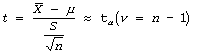 Step # 03: State the test statistic (n<30)
t-test statistic
Step # 04: Computation/ calculation of test statistic


Data
µ = 22
S = 5
n = 16


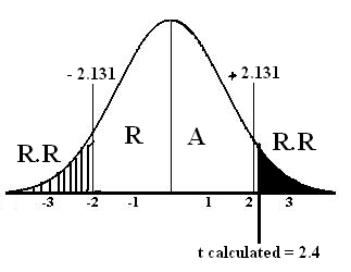
t calculated = 2.4
Step # 05: Find Critical Value or Rejection (critical) Region
 For critical value we find and on the basis of its answer we see critical value from t-distribution table.
Critical value = α/2(v = 16-1)
= 0.05/2(v = 15)
= (0.025, 15)
t tabulated = ± 2.131
t calculated = 2.4
Step # 06: Conclusion: Since t calculated = 2.4 falls in the region of rejection therefore we reject at the 5% level of significance. There is sufficient evidence to conclude that Population mean is not equal to 22.
Z- TEST
- Z-test is applied when the distribution is normal and the population standard deviation σ is known or when the sample size n is large (n ≥ 30) and with unknown σ (by taking S as estimator of σ).
- Z-test is used to test hypotheses about μ when the population standard deviation is known and population distribution is normal or sample size is large (n ≥ 30)
Calculating one sample z-test
Example: A random sample of size 49 with mean 32 is taken from a normal population whose standard deviation is 4. Test at 5% LOS that : µ= 25
: µ≠25
SOLUTION
Step # 01: : µ= 25
: µ≠25
Step # 02: α = 0.05
Step # 03:Since (n<30), we apply z-test statistic
Step # 04: Calculation of test statistic


Data
µ = 25
= 4
n = 49


Zcalculated = 12.28
Step # 05: Find Critical Value or Rejection (critical) Region
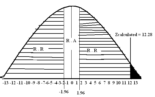
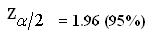
Critical Value (5%) (2-tail) = ±1.96
Zcalculated = 12.28
Step # 06: Conclusion: Since Zcalculated = 12.28 falls in the region of rejection therefore we reject at the 5% level of significance. There is sufficient evidence to conclude that Population mean is not equal to 25.
CHI-SQUARE
A statistic which measures the discrepancy (difference) between KObserved Frequencies fo1, fo2… fok and the corresponding ExpectedFrequencies fe1, fe2……. fek
The chi-square is useful in making statistical inferences about categorical data in whichthe categories are two and above.
Characteristics
- Every χ2 distribution extends indefinitely to the right from 0.
- Every χ2 distribution has only one (right sided) tail.
- As df increases, the χ2 curves get more bell shaped and approach the normal curve in appearance (but remember that a chi square curvestarts at 0, not at – ∞ )
Calculating Chi-Square
Example 1: census of U.S. determine four categories of doctors practiced in different areas as
| Specialty |
% |
Probability |
| General Practice |
18% |
0.18 |
| Medical |
33.9 % |
0.339 |
| Surgical |
27 % |
0.27 |
| Others |
21.1 % |
0.211 |
| Total |
100 % |
1.000 |
A searcher conduct a test after 5 years to check this data for changes and select 500 doctors and asked their speciality. The result were:
| Specialty |
frequency |
| General Practice |
80 |
| Medical |
162 |
| Surgical |
156 |
| Others |
102 |
| Total |
500 |
Hypothesis testing:
Step 01”
Null Hypothesis (Ho):
There is no difference in specialty distribution (or) the current specialty distribution of US physician is same as declared in the census.
Alternative Hypothesis (HA):
There is difference in specialty distribution of US doctors. (or) the current specialty distribution of US physician is different as declared in the census.
Step 02: Level of Significance
α = 0.05
Step # 03:Chi-squire Test Statistic
Step # 04:
Statistical Calculation
fe (80) = 18 % x 500 = 90
fe (162) = 33.9 % x 500 = 169.5
fe (156) = 27 % x 500 = 135
fe (102) = 21.1 % x 500 = 105.5
| S # (n) |
Specialty |
fo |
fe |
(fo – fe) |
(fo – fe) 2 |
(fo – fe) 2 / fe |
| 1 |
General Practice |
80 |
90 |
-10 |
100 |
1.11 |
| 2 |
Medical |
162 |
169.5 |
-7.5 |
56.25 |
0.33 |
| 3 |
Surgical |
156 |
135 |
21 |
441 |
3.26 |
| 4 |
Others |
102 |
105.5 |
-3.5 |
12.25 |
0.116 |
|
|
|
4.816 |
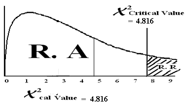 χ2cal= = 4.816
Step # 05:
Find critical region using X2– chi-squire distribution table
χ2 = χ2 = χ2 = 7.815
tab (α,d.f) (0.05,3)
(d.f = n – 1)
Step # 06:
Conclusion: Since χ2cal value lies in the region of acceptance therefore we accept the HO and reject HA. There is no difference in specialty distribution among U.S. doctors.
Example2: A sample of 150 chronic Carriers of certain antigen and a sample of 500 Non-carriers revealed the following blood group distributions. Can one conclude from these data that the two population from which samples were drawn differ with respect to blood group distribution? Let α = 0.05.
| Blood Group |
Carriers |
Non-carriers |
Total |
| O |
72 |
230 |
302 |
| A |
54 |
192 |
246 |
| B |
16 |
63 |
79 |
| AB |
8 |
15 |
23 |
| Total |
150 |
500 |
650 |
Hypothesis Testing
Step # 01: HO: There is no association b/w Antigen and Blood Group
HA: There is some association b/w Antigen and Blood Group
Step # 02:α = 0.05
Step # 03:Chi-squire Test Statistic
Step # 04:
Calculation
fe (72) = 302*150/650 = 70
fe (230) = 302*500/ 650 = 232
fe (54) = 246*150/650 = 57
fe (192) = 246*500/650 = 189
fe (16) = 79*150/650 = 18
fe (63) = 79*500/650 = 61
fe (8) = 23*150/650 = 05
fe (15) = 23*500/650 = 18
| fo |
fe |
(fo – fe) |
(fo – fe) 2 |
(fo – fe) 2 / fe |
| 72 |
70 |
2 |
4 |
0.0571 |
| 230 |
232 |
-2 |
4 |
0.0172 |
| 54 |
57 |
-3 |
9 |
0.1578 |
| 192 |
189 |
3 |
9 |
0.0476 |
| 16 |
18 |
-2 |
4 |
0.2222 |
| 63 |
61 |
2 |
4 |
0.0655 |
| 8 |
5 |
3 |
9 |
1.8 |
| 15 |
18 |
-3 |
9 |
0.5 |
|
2.8674 |
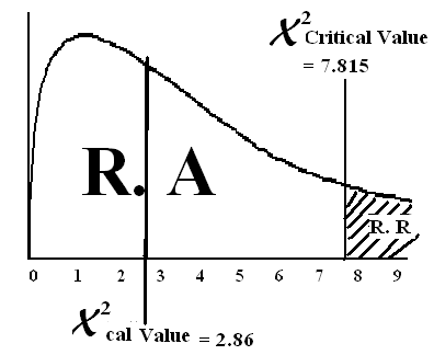 X2 = = 2.8674
X2cal = 2.8674
Step # 05:
Find critical region using X2– chi-squire distribution table
X2 = (α, d.f) = (0.05, 3) = 7.815
Step # 06:
Conclusion: Since X2cal value lies in the region of acceptance therefore we accept the HO andreject HA. Means There is no association b/w Antigen and Blood Group
WHAT IS TEST OF SIGNIFICANCE? WHY IT IS NECESSARY? MENTION NAMES OF IMPORTANT TESTS.
1. Test of significance
A procedure used to establish the validity of a claim by determining whether or not the test statistic falls in the critical region. If it does, the results are referred to as significant. This test is sometimes called the hypothesis test.
The methods of inference used to support or reject claims based on sample data are known as tests of significance.
Why it is necessary
A significance test is performed;
- To determine if an observed value of a statistic differs enough from a hypothesized value of a parameter
- To draw the inference that the hypothesized value of the parameter is not the true value. The hypothesized value of the parameter is called the “null hypothesis.”
Types of test of significance
- Parametric
- t-test (one sample & two sample)
- z-test (one sample & two Sample)
- F-test.
- Non-parametric
- Chi-squire test
- Mann-Whitney U test
- Coefficient of concordance (W)
- Median test
- Kruskal-Wallis test
- Friedman test
- Rank difference methods (Spearman rho and Kendal’s tau)
P –Value:
A p-value is the probability that the computed value of a test statistic is at least as extreme as a specified value of the test statistic when the null hypothesis is true. Thus, the p value is the smallest value of for which we can reject a null hypothesis.
Simply the p value for a test may be defined also as the smallest value of α for which the null hypothesis can be rejected.
The p value is a number that tells us how unusual our sample results are, given that the null hypothesis is true. A p value indicating that the sample results are not likely to have occurred, if the null hypothesis is true, provides justification for doubting the truth of the null hypothesis.
Test Decisions with p-value
The decision about whether there is enough evidence to reject the null hypothesis can be made by comparing the p-values to the value of α, the level of significance of the test.
A general rule worth remembering is:
- If the p value is less than or equal to, we reject the null hypothesis
- If the p value is greater than, we do not reject the null hypothesis.
| If p-value ≤ α reject the null hypothesis |
| If p-value ≥ α fail to reject the null hypothesis |
Observational Study:
An observational study is a scientific investigation in which neither the subjects under study nor any of the variables of interest are manipulated in any way.
An observational study, in other words, may be defined simply as an investigation that is not an experiment. The simplest form of observational study is one in which there are only two variables of interest. One of the variables is called the risk factor, or independent variable, and the other variable is referred to as the outcome, or dependent variable.
Risk Factor:
The term risk factor is used to designate a variable that is thought to be related to some outcome variable. The risk factor may be a suspected cause of some specific state of the outcome variable.
Types of Observational Studies
There are two basic types of observational studies, prospective studies and retrospective studies.
Prospective Study:
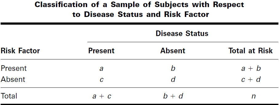
A prospective study is an observational study in which two random samples of subjects are selected. One sample consists of subjects who possess the risk factor, and the other sample consists of subjects who do not possess the risk factor. The subjects are followed into the future (that is, they are followed prospectively), and a record is kept on the number of subjects in each sample who, at some point in time, are classifiable into each of the categories of the outcome variable.
The data resulting from a prospective study involving two dichotomous variables can be displayed in a 2 x 2 contingency table that usually provides information regarding the number of subjects with and without the risk factor and the number who did and did not
Retrospective Study:
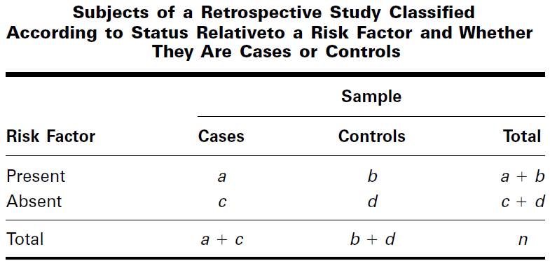
A retrospective study is the reverse of a prospective study. The samples are selected from those falling into the categories of the outcome variable. The investigator then looks back (that is, takes a retrospective look) at the subjects and determines which ones have (or had) and which ones do not have (or did not have) the risk factor.
From the data of a retrospective study we may construct a contingency table
Relative Risk:
Relative risk is the ratio of the risk of developing a disease among subjects with the risk factor to the risk of developing the disease among subjects without the risk factor.
We represent the relative risk from a prospective study symbolically as
We may construct a confidence interval for RR
100 (1 – α)%CI=
Where zα is the two-sided z value corresponding to the chosen confidence coefficient and X2is computed by Equation
Interpretation of RR
- The value of RR may range anywhere between zero and infinity.
- A value of 1 indicates that there is no association between the status of the risk factor and the status of the dependent variable.
- A value of RR greater than 1 indicates that the risk of acquiring the disease is greater among subjects with the risk factor than among subjects without the risk factor.
- An RR value that is less than 1 indicates less risk of acquiring the disease among subjects with the risk factor than among subjects without the risk factor.
EXAMPLE
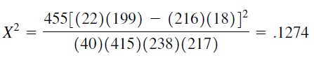
In a prospective study of pregnant women, Magann et al. (A-16) collected extensive information on exercise level of low-risk pregnant working women. A group of 217 women did no voluntary or mandatory exercise during the pregnancy, while a group of
238 women exercised extensively. One outcome variable of interest was experiencing preterm labor. The results are summarized in Table
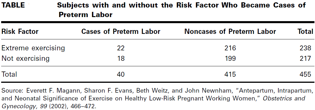
Estimate the relative risk of preterm labor when pregnant women exercise extensively.
Solution:
By Equation
These data indicate that the risk of experiencing preterm labor when a woman exercises heavily is 1.1 times as great as it is among women who do not exercise at all.
Confidence Interval for RR
We compute the 95 percent confidence interval for RR as follows.
The lower and upper confidence limits are, respectively
= 0.65 and = 1.86
Conclusion:
Since the interval includes 1, we conclude, at the .05 level of significance, that the population risk may be 1. In other words, we conclude that, in the population, there may not be an increased risk of experiencing preterm labor when a pregnant woman exercises extensively.
Odds Ratio
An odds ratio (OR) is a measure of association between an exposure and an outcome. The OR represents the odds that an outcome will occur given a particular exposure, compared to the odds of the outcome occurring in the absence of that exposure.
It is the appropriate measure for comparing cases and controls in a retrospective study.
Odds:
The odds for success are the ratio of the probability of success to the probability of failure.
Two odds that we can calculate from data displayed as in contingency Table of retrospective study
- The odds of being a case (having the disease) to being a control (not having the disease) among subjects with the risk factor is [a/ (a +b)] / [b/ (a + b)] = a/b
- The odds of being a case (having the disease) to being a control (not having the disease) among subjects without the risk factor is [c/(c +d)] / [d/(c + d)] = c/d
The estimate of the population odds ratio is
We may construct a confidence interval for OR by the following method:
100 (1 – α) %CI=
Where is the two-sided z value corresponding to the chosen confidence coefficient and X2 is computed by Equation
Interpretation of the Odds Ratio:
In the case of a rare disease, the population odds ratio provides a good approximation to the population relative risk. Consequently, the sample odds ratio, being an estimate of the population odds ratio, provides an indirect estimate of the population relative risk in the case of a rare disease.
- The odds ratio can assume values between zero and ∞.
- A value of 1 indicates no association between the risk factor and disease status.
- A value less than 1 indicates reduced odds of the disease among subjects with the risk factor.
- A value greater than 1 indicates increased odds of having the disease among subjects in whom the risk factor is present.
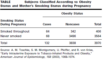
EXAMPLE
Toschke et al. (A-17) collected data on obesity status of children ages 5–6 years and the smoking status of the mother during the pregnancy. Table below shows 3970 subjects classified as cases or noncases of obesity and also classified according to smoking status of the mother during pregnancy (the risk factor).
We wish to compare the odds of obesity at ages 5–6 among those whose mother smoked throughout the pregnancy with the odds of obesity at age 5–6 among those whose mother did not smoke during pregnancy.
Solution
By formula:
We see that obese children (cases) are 9.62 times as likely as nonobese children (noncases) to have had a mother who smoked throughout the pregnancy.
We compute the 95 percent confidence interval for OR as follows.
The lower and upper confidence limits for the population OR, respectively, are
= 7.12 and = = 13.00
We conclude with 95 percent confidence that the population OR is somewhere between
7.12 And 13.00. Because the interval does not include 1, we conclude that, in the population, obese children (cases) are more likely than nonobese children (noncases) to have had a mother who smoked throughout the pregnancy.

 Formula
OR S2 =
Calculating variance: Heart rate of certain patient is 80, 84, 80, 72, 76, 88, 84, 80, 78, & 78. Calculate variance for this data.
Solution:
Step 1:
Find mean of this data
Formula
OR S2 =
Calculating variance: Heart rate of certain patient is 80, 84, 80, 72, 76, 88, 84, 80, 78, & 78. Calculate variance for this data.
Solution:
Step 1:
Find mean of this data
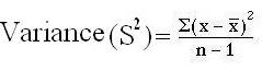 Variance = 184/ 10-1 = 184/9
Variance = 20.44
Standard Deviation
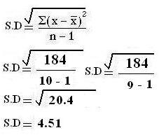
Variance = 184/ 10-1 = 184/9
Variance = 20.44
Standard Deviation
 Formula:
OR S =
Calculating Standard Deviation (we use same example): Heart rate of certain patient is 80, 84, 80, 72, 76, 88, 84, 80, 78, & 78. Calculate standard deviation for this data.
SOLUTION:
Step 1: Find mean of this data
Formula:
OR S =
Calculating Standard Deviation (we use same example): Heart rate of certain patient is 80, 84, 80, 72, 76, 88, 84, 80, 78, & 78. Calculate standard deviation for this data.
SOLUTION:
Step 1: Find mean of this data
 MERITS AND DEMERITS OF STD. DEVIATION


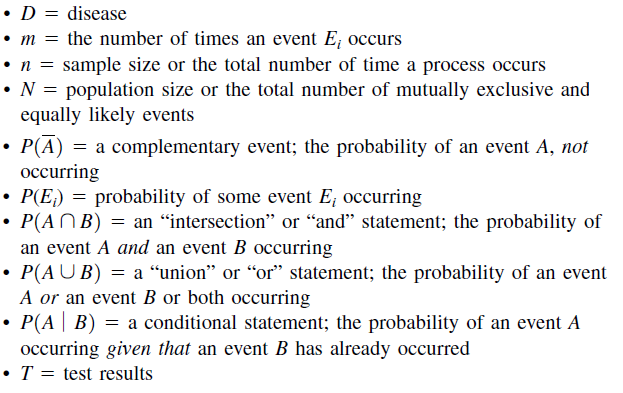
 Symbol Key:


 Formula
 Formula:


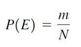 If an event can occur in N mutually exclusive and equally likely ways, and if m of these possess a trait E, the probability of the occurrence of E expressed as:
 Rule 2: When two events are dependent, the probability of both events occurring is P (A and B) =P (A) x P (B|A), where P (B|A) is the probability that event B occurs given that event A has already occurred.
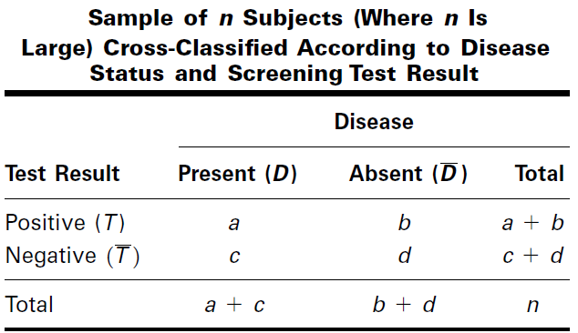 A false negative results when a test indicates a negative status when the true status is positive.
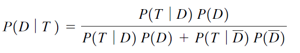 The predictive value positive of a screening test (or symptom) is the probability that a subject has the disease given that the subject has a positive screening test result (or has the symptom).
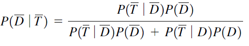 The predictive value negative of a screening test (or symptom) is the probability that a subject does not have the disease, given that the subject has a negative screening test result (or does not have the symptom).
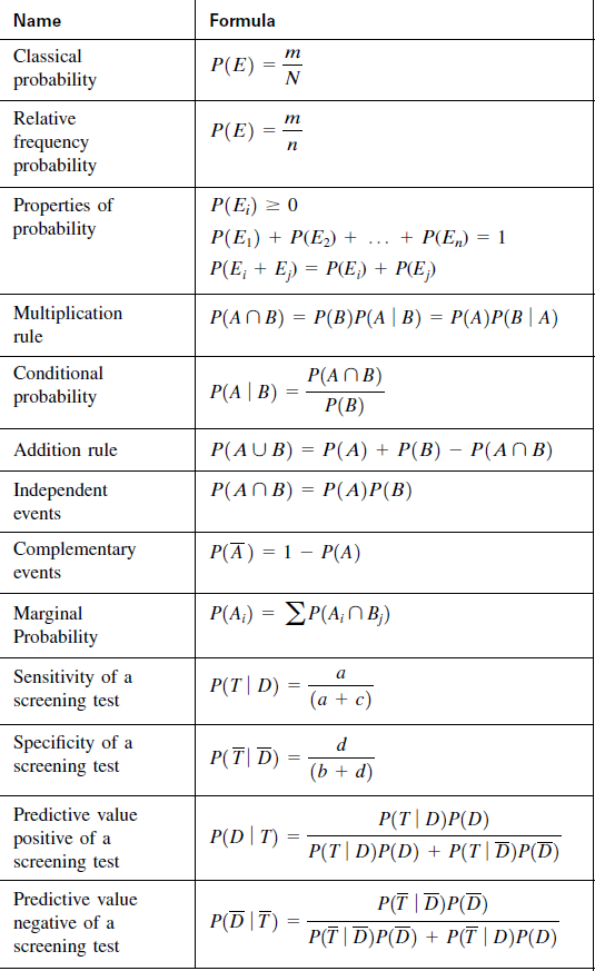
 Repetition of same items with different arrangement is allowed.
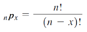 Examples
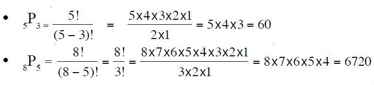
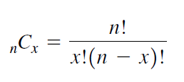 Repetition of same objects in not allowed with different arrangement