Measure of Central Tendency
Central tendency or central position or statistical averages reflects the central point or the most characteristic value of a set of measurements. The measure of central tendency describes the one score that best represents the entire distribution,
(OR)
A single figure that describes the entire series of observations with their varying sizes, occupying a central position.
The most common measures of central tendency are
Characteristics of Central Tendency:
-
It should be rigidly defined
-
An average should be properly defined so that it has one and only one interpretation.
-
The average should not depend on the personal prejudice and bias of the investigator.
-
It should be based onall items
-
It should be easily understand.
-
It should not be unduly affected by the extreme value.
-
It should be least affected by the fluctuation of the sampling.
-
It should be easy to interpret.
-
It should be easily subjected to further mathematical calculations.
Measure of Central Tendency
If n ≤ 15
Direct Method
If n > 15
Frequency Distribution Method
Simple /Ungrouped Frequency Distribution
(Range ≤ 20 digits)
Grouped Frequency Distribution
(Range > 20 digits)
Mean:
It is defined as a value which is obtained by dividing the sum of all the values by the numbers of observations. Thus arithmetic mean of a set of values x1, x2, x3, x4.. . . .xn is denoted by (read as “x bar”) and is calculated as:
= = (Direct Method)
Where sign ∑ stands for the sum and “n” is the number of observations.
Example:
The grades of a student in five examinations were 67, 75, 81, 87, 90 find the arithmetic mean of grades.
Solution:
=
=
Here, = = 80
Thus, the mean grade is 80.
Method of Finding Mean
If x1, x2, x3, x4, ….xn are the values of different observations andf1, f2, f3, f4, ….fnare their frequencies, then,
=
Or. A.M. =
Example 2. The number of children of 80 families in a village are given below:
| No. of Children/Family |
1 |
2 |
3 |
4 |
5 |
6 |
| No. of Families |
8 |
10 |
10 |
25 |
20 |
7 |
Calculate mean.
Solution: let xi represent the number of children per family and fi represent the number of families. The calculations are presented in the following table:
| No. of Children/Family
(xi) |
No. of Families
(fi) |
fixi |
|
1 |
8 |
8 |
|
2 |
10 |
20 |
|
3 |
10 |
30 |
|
4 |
25 |
100 |
|
5 |
20 |
100 |
|
6 |
7 |
42 |
|
n=∑fi =80 |
∑fixi = 300 |
Thus = = = 3.75
Methods of Finding Arithmetic mean for Grouped Data
Let x1, x2, x3, x4.. . . .xnbe mid-points of the class intervals with corresponding frequencies f1, f2, f3, f4, ….fn . Then the arithmetic mean is obtained by dividing the sum of the product of “f “ and “x” by the total of all frequencies.
Thus:
A.M. = =
=
Example:
Given below are the heights of (in inches) of 200 students. Find A.M.
| Height (inches) |
30-35 |
35-40 |
40-45 |
45-50 |
50-55 |
55-60 |
| No. of Students |
28 |
32 |
36 |
46 |
36 |
22 |
Solution:
| Height
(Inches) |
Mid points
(x) |
Frequency
(f) |
fx |
|
30-35 |
32.5 |
28 |
910 |
|
35-40 |
37.5 |
32 |
1200 |
|
40-45 |
42.5 |
36 |
1530 |
|
45-50 |
47.5 |
46 |
2185 |
|
50-55 |
52.5 |
36 |
1890 |
|
55-60 |
57.5 |
22 |
1265 |
|
Total: |
— |
∑f = 200 |
∑fx = 8980 |
= = = 44.90 (inches).
Example: Given below are the weights (in kgs) of 100 students. Find Mean Weight:
| Weight |
70-74 |
75-79 |
80-84 |
85-89 |
90-94 |
| No. of Students |
10 |
24 |
46 |
12 |
8 |
Solution:
| Weight
(Kg) |
Mid-Points
(x) |
Frequency
(f) |
fx |
|
70 – 74 |
72 |
10 |
720 |
|
75 – 79 |
77 |
24 |
1848 |
|
80 – 84 |
82 |
46 |
3772 |
|
85 – 89 |
87 |
12 |
1044 |
|
90 – 94 |
92 |
8 |
736 |
|
Total: |
— |
∑f = 100 |
∑fx = 8120 |
= = = 81.20
Here, Mean Weight is 31.2 kgs.
Merits of Mean
-
It has the simplest average formula which is easily understandable and easy to compute.
-
It is so rigidly defined by mathematical formula that everyone gets same result for single problem.
-
Its calculation is based on all the observations.
-
It is least affected by sampling fluctuations.
-
It is a typical i.e. it balances the value at either side.
-
It is the best measure to compare two or more series.(data)
-
Mean is calculated on value and does not depend upon any position.
-
Mathematical centre of a distribution
-
Good for interval & ratio scale
-
Does not ignore any information
-
Inferential statistics is based on mathematical properties of the mean.
-
It is based on all the observations.
-
It is easy to calculate and simple to understand.
-
It is relatively stable and amendable to mathematical treatment.
Demerits of Mean
-
It cannot be calculated if all the values are not known.
-
The extreme values have greater affect on it.
-
It cannot be determined for the qualitative data.
-
It may not exist in data.
Median:
It is the middle most point or the central value of the variable in a set of observation when observations are arranged in either order of their magnitudes.
It is the value in a series, which divides the series into two equal parts, one consisting of all values less and the other all values greater than it.
Median for Ungrouped data
Median of “n” observations, x1, x2, x3,…xn can be obtained as follows:
-
When “n” is an odd number,
Median = ()th observation
-
When “n” is an even number,
Median is the average of ()thand ()thobservations.
Or
Simply use ()th observation. It will the average
The median for the discrete frequency distribution can be obtained as above, Using a cumulative frequency distribution.
Problem
Find the median of the following data:
12, 2, 16, 8, 14, 10, 6
Step 1: Organize the data, or arrange the numbers from smallest to largest.
2, 6, 8, 10, 12, 14, 16
Step 2: count number of observation in data (n)
.n = 7
Step 3: Since the number of data values is odd, the median will be found in the position.
Median term (m) =

7 + 1 8
= = = 4th value
2 2
Step 4: In this case, the median is the value that is found in the fourth position of the organized data, therefore
Median = 10
Problem
Median for even data:
Find the median of the following data:
7, 9, 3, 4, 11, 1, 8, 6, 1, 4
Step 1: Organize the data, or arrange the numbers from smallest to largest.
1, 1, 3, 4, 4, 6, 7, 8, 9, 11
Step 2: Since the number of data values is even, the median will be the mean value of the numbers found before and after the

position.
Step 3: The number found before the 5.5 position is 4 and the number found after the 5.5 position is 6. Now, you need to find the mean value.
1, 1, 3, 4, 4, 6, 7, 8, 9, 11

Example:
The following are the runs made by a batsman in 7 matches:
8, 12, 18, 13, 16, 5, 20.Find the median.
Solution: Writing the runs in ascending order.
5, 8, 12, 13, 16, 18, 20
As n=7
Median= ()thitem = ()4th item.
Hence, Median is13 runs.
Example:
Following are the marks (out of 100) obtained by 10 students in English:
23, 15, 35, 41, 48, 5, 8, 9, 11, 51. Find the median mark.
Solution: arranging the marks in ascending order. The marks are:
5, 8, 9, 11, 15, 23, 35, 41, 48, 51
As n= 10
So, median = [] item.
=
Or, Median = [15+23] = = 19 marks.
Alternative Method:
Median term(m) = ()th value
=
= 11/2 = 5.5th value
5, 8, 9, 11, 15, 23, 35, 41, 48, 51
M1 M2
Median =
Median = = 19
Median for Grouped data
It is obtained by the following formula:
Median = l1 +()
Where, l1 = lower class limit of median class.
l2 = upper class limit of median class
f = frequency of median class.
m = or
C = cumulative frequency preceding the median class.
n = total frequency, i.e. ∑f.
Example:
Find the median height of 200 students in given data
Solution:
| Class interval |
Frequency (f) |
C.F |
|
30-35 |
28 |
28 |
|
35-40 |
32 |
28+32=60 |
|
40-45 |
36 |
60+36=96 |
| 45-50 |
46 |
96+46=142 |
|
50-55 |
36 |
142+36=178 |
|
55-60 |
22 |
178+22=200 n |
Median =
As 100.5 th item lies in (45-50), it is the median class with l1 = 45, l2 = 50 ,f= 46, C= 96
Median = l1 +()
Median = 45 + (
= 45 +
= 45 + 0.489
= 45.489
Thus, median height is 45.489 inches.
2nd Method:
l + (
Where, l = lower class boundary of median class.
w = width of median class.
f = frequency of median class.
n = total frequency, i.e. ∑f.
c = cumulative frequency preceding the median class.
Example:
Following are the weights in kgs of 100 students. Find the median weight.
| Weights (kgs) |
70-74 |
75-79 |
80-84 |
85-89 |
90-94 |
| No of students. |
10 |
24 |
46 |
12 |
8 |
Solution: As class boundaries are not given so, first of all we make class boundaries by using procedure.
| Weight (kgs) |
No. of students |
Class boundaries |
C.F |
|
70-74 |
10 |
69.5-74.5 |
10 |
|
75-80 |
24 |
74.5-79.5 |
34 |
|
80-84 |
46 |
79.5-84.5 |
80 |
|
85-89 |
12 |
84.5-89.5 |
92 |
|
90-94 |
8 |
89.5-94.5 |
100 |
Median =
As 50th item lies in (79.5-84.5), it is the median class with h= 5, f= 46, C= 34
Median = l + (, we find
Median = 79.5 + (
= 79.5 +
Hence, median weight is 81.24 kg.
Merits of Median:
-
It is easily understood although it is not so popular as mean.
-
It is not influenced or affected by the variation in the magnitude or the extremes items.
-
The value of the median can be graphically ascertained by ogives.
-
It is the best measure for qualitative data such as beauty, intelligence etc.
-
The median indicated the value of middle item in the distribution i.e. middle most item is the median
-
It can be determined even by inspection in many cases.
-
Good with ordinal data
-
Easier to compute than the mean
Demerits of Median:
-
For the calculation of median, data must be arranged.
-
Median being a positional average, cannot be dependent on each and every observations.
-
It is not subject to algebraic treatment.
-
Median is more affected or influenced by samplings fluctuations that the arithmetic mean.
-
May not exist in data.
-
It is not rigorously defined.
-
It does not use values of all observations.
Mode:
Mode is considered as the value in a series which occurs most frequently (has the highest frequency)
The mode of distribution is the value at the point around which the items tend to be most heavily concentrated. It may be regarded as the most typical value.
-
The word modal is often used when referring to the mode of a data set.
-
If a data set has only one value that occurs most often, the set is called unimodal.
-
A data set that has two values that occur with the same greatest frequency is referred to as bimodal.
-
When a set of data has more than two values that occur with the same greatest frequency, the set is called multimodal.
Mode for Ungrouped data
Example 1. The grades of Jamal in eight monthly tests were 75, 76, 80, 80, 82, 82, 82, 85.Find the mode of his grades.
Solution: As 82 is repeated more than any other number, so clearly mode is 82.
Example 2. Ten students were asked about the number of questions they have solved out of 20 questions, last week. Records were 13, 14, 15, 11, 16, 10, 19, 20, 18, 17. Find the modes.
Solution: it is obvious that the data contain no mode, as none of the numbers is repeated. Sometimes data contains several modes.
If x = 10, 15, 15, 15, 20, 20, 20, 25 then the data contains two modes i.e. 15 and 20.
Mode for grouped data
Mode for the grouped data can be calculated by the following formula:
Mode=
(OR)
Mode=
(OR)
Mode=
l1= lower limit (class boundary) of the modal class.
l2 = upper limit of the modal class
fm= frequency of the modal class
f1= frequency associated with the class preceding the modal class.
f2 = frequency associated with the class following the modal class
h = (size of modal class)
The class with highest frequency is called the “Modal Class”.
Example 3. Find the mode for the heights of 200 students in given data
| Height (inches) |
Frequency |
|
30-35 |
28 |
|
35-40 |
32 |
|
40-45 |
36 () |
| 45-50 |
46 () |
|
50-55 |
36 () |
|
55-60 |
22 |
|
∑f=200 |
Solution:
Mode=
Mode=
Mode=
Mode=
Mode=
Mode=
Mode = 47. 5
Merits of Mode:
-
It can be obtained by inspection.
-
It is not affected by extreme values.
-
This average can be calculated from open end classes.
-
The score comes from the data set
-
Good for nominal data
-
Good when there are two ‘typical‘ scores
-
Easiest to compute and understand
-
It can be used to describe qualitative phenomenon
-
The value of mode can also be found graphically.
Demerits of Mode
-
Mode has no significance unless a large number of observations are available.
-
It cannot be treated algebraically.
-
It is a peculiar measure of central tendency.
-
For the calculation of mode, the data must be arranged in the form of frequency distribution.
-
It is not rigidly define measure.
-
Ignores most of the information in a distribution
-
Small samples may not have a mode.
-
It is not based on all the observations.
Empirical Relationship b/w
Skewness:
Data distributions may be classified on the basis of whether they are symmetric or asymmetric. If a distribution is symmetric, the left half of its graph (histogram or frequency polygon) will be a mirror image of its right half. When the left half and right half of the graph of a distribution are not mirror images of each other, the distribution is asymmetric.
If the graph (histogram or frequency polygon) of a distribution is asymmetric, the distribution is said to be skewed. The mean, median and mode do not fall in the middle of the distribution.
Types of Skewness
- Positive skewness: If a distribution is not symmetric because its graph extends further to the right than to the left, that is, if it has a long tail to the right, we say that the distribution is skewed to the right or is positively skewed. In positively skewed distribution Mean > Median > Mode. The positive skewness indicates that the mean is more influenced than the median and mode, by the few extremely high value. Positively skewed distribution have positive value because mean is greater than mode
- Negative skewness: If a distribution is not symmetric because its graph extends further to the left than to the right, that is, if it has a long tail to the left, we say that the distribution is skewed to the left or is negatively skewed. In negatively skewed distribution Mean < Median < Mode. Negatively skewed distribution have negative value because mean is less than mode.
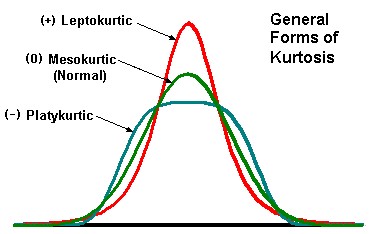
KURTOSIS
Kurtosis is a measure of the degree to which a distribution is “peaked” or flat in comparison to a normal distribution whose graph is characterized by a bell-shaped appearance.
- Platykurtic curve: when the frequency distribution curve is flatter than the normal bell shaped curve
- Leptokurtic curve: when the frequency distribution curve is more peaked than the normal bell shaped curve
- Mesokurtic curve: the normal bell shaped distribution curve.
|
 |

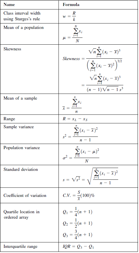
 Formula
 Formula: