This term is used commonly to mean scatter, Deviation, Fluctuation, Spread or variability of data.
The degree to which the individual values of the variate scatter away from the average or the central value, is called a dispersion.
Types of Measures of Dispersions:
- Absolute Measures of Dispersion: The measures of dispersion which are expressed in terms of original units of a data are termed as Absolute Measures.
- Relative Measures of Dispersion: Relative measures of dispersion, are also known as coefficients of dispersion, are obtained as ratios or percentages. These are pure numbers independent of the units of measurement and used to compare two or more sets of data values.
Absolute Measures
- Range
- Quartile Deviation
- Mean Deviation
- Standard Deviation
Relative Measure
- Co-efficient of Range
- Co-efficient of Quartile Deviation
- Co-efficient of mean Deviation
- Co-efficient of Variation.
The Range:
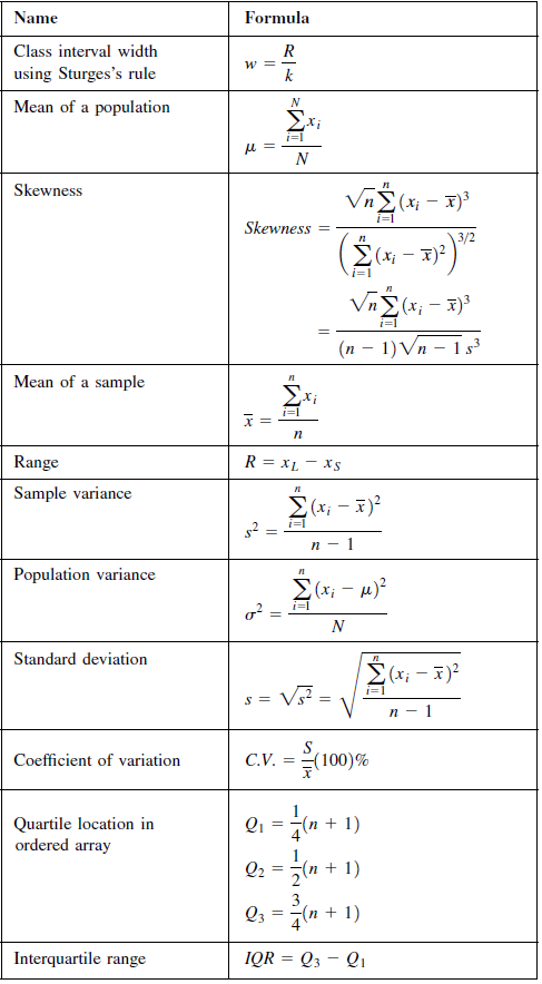
1. The range is the simplest measure of dispersion. It is defined as the difference between the largest value and the smallest value in the data:
2. For grouped data, the range is defined as the difference between the upper class boundary (UCB) of the highest class and the lower class boundary (LCB) of the lowest class.
MERITS OF RANGE:-
- Easiest to calculate and simplest to understand.
- Gives a quick answer.
DEMERITS OF RANGE:-
- It gives a rough answer.
- It is not based on all observations.
- It changes from one sample to the next in a population.
- It can’t be calculated in open-end distributions.
- It is affected by sampling fluctuations.
- It gives no indication how the values within the two extremes are distributed
Quartile Deviation (QD):
1. It is also known as the Semi-Interquartile Range. The range is a poor measure of dispersion where extremely large values are present. The quartile deviation is defined half of the difference between the third and the first quartiles:
QD = Q3 – Q1/2
Inter-Quartile Range
The difference between third and first quartiles is called the ‘Inter-Quartile Range’.
IQR = Q3 – Q1
Mean Deviation (MD):
1. The MD is defined as the average of the deviations of the values from an average:
It is also known as Mean Absolute Deviation.
2. MD from median is expressed as follows:

3. for grouped data:


Mean Deviation:
- The MD is simple to understand and to interpret.
- It is affected by the value of every observation.
- It is less affected by absolute deviations than the standard deviation.
- It is not suited to further mathematical treatment. It is, therefore, not as logical as convenient measure of dispersion as the SD.
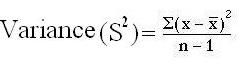
The Variance:
- Mean of all squared deviations from the mean is called as variance
- (Sample variance=S2; population variance= σ2sigma squared (standard deviation squared). A high variance means most scores are far away from the mean, a low variance indicates most scores cluster tightly about the mean.
 Formula
OR S2 =
Calculating variance: Heart rate of certain patient is 80, 84, 80, 72, 76, 88, 84, 80, 78, & 78. Calculate variance for this data.
Solution:
Step 1:
Find mean of this data

= 800/10 Mean = 80
Step 2:
Draw two Columns respectively ‘X’ and deviation about mean (X-  ). In column ‘X’ put all values of X and in (X-
  ) subtract each ‘X’ value with
  .
.
Step 3:
Draw another Column of (X-  ) 2, in which put square of deviation about mean.
| X |
(X-  ) )
Deviation about mean |
(X-  )2 )2
Square of Deviation about mean |
| 80
84
80
72
76
88
84
80
78
78 |
80 – 80 = 0
84 – 80 = 4
80 – 80 = 0
72 – 80 = -8
76 – 80 = -4
88 – 80 = 8
84 – 80 = 4
80 – 80 = 0
78 – 80 = -2
78 – 80 = -2 |
0 x 0 = 00
4 x 4 = 16
0 x 0 = 00
-8 x -8 = 64
-4 x -4 = 16
8 x 8 = 64
4 x 4 = 16
0 x 0 = 00
-2 x -2 = 04
-2 x -2 = 04 |
| ∑X = 800
 = 80 = 80
|
∑(X-  ) = 0 ) = 0
Summation of Deviation about mean is always zero |
∑(X-  )2 = 184 )2 = 184
Summation of Square of Deviation about mean |
Step 4
Apply formula and put following values
∑(X-  ) 2= 184
n = 10

Variance = 184/ 10-1 = 184/9
Variance = 20.44
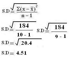
Standard Deviation
- The SD is defined as the positive Square root of the mean of the squared deviations of the values from their mean.
- The square root of the variance.
- It measures the spread of data around the mean. One standard deviation includes 68% of the values in a sample population and two standard deviations include 95% of the values & 3 standard deviations include 99.7% of the values
- The SD is affected by the value of every observation.
- In general, it is less affected by fluctuations of sampling than the other measures of dispersion.
- It has a definite mathematical meaning and is perfectly adaptable to algebraic treatment.
 Formula:
OR S =
Calculating Standard Deviation (we use same example): Heart rate of certain patient is 80, 84, 80, 72, 76, 88, 84, 80, 78, & 78. Calculate standard deviation for this data.
SOLUTION:
Step 1: Find mean of this data

= 800/10 Mean = 80
Step 2:
Draw two Columns respectively ‘X’ and deviation about mean (X-). In column ‘X’ put all values of X and in (X-) subtract each ‘X’ value with.
Step 3:
Draw another Column of (X- ) 2, in which put square of deviation about mean.
| X |
(X-  ) )
Deviation about mean |
(X-  )2 )2
Square of Deviation about mean |
| 80
84
80
72
76
88
84
80
78
78 |
80 – 80 = 0
84 – 80 = 4
80 – 80 = 0
72 – 80 = -8
76 – 80 = -4
88 – 80 = 8
84 – 80 = 4
80 – 80 = 0
78 – 80 = -2
78 – 80 = -2 |
0 x 0 = 00
4 x 4 = 16
0 x 0 = 00
-8 x -8 = 64
-4 x -4 = 16
8 x 8 = 64
4 x 4 = 16
0 x 0 = 00
-2 x -2 = 04
-2 x -2 = 04 |
| ∑X = 800
 = 80 = 80
|
∑(X-  ) = 0 ) = 0
Summation of Deviation about mean is always zero |
∑(X-  )2 = 184 )2 = 184
Summation of Square of Deviation about mean |
Step 4
Apply formula and put following values
∑(X-  )2 = 184
n = 10

MERITS AND DEMERITS OF STD. DEVIATION
- Std. Dev. summarizes the deviation of a large distribution from mean in one figure used as a unit of variation.
- It indicates whether the variation of difference of a individual from the mean is real or by chance.
- Std. Dev. helps in finding the suitable size of sample for valid conclusions.
- It helps in calculating the Standard error.
DEMERITS-
- It gives weightage to only extreme values. The process of squaring deviations and then taking square root involves lengthy calculations.
Relative measure of dispersion:
(a) Coefficient of Variation,
(b) Coefficient of Dispersion,
(c) Quartile Coefficient of Dispersion, and
(d) Mean Coefficient of Dispersion.
Coefficient of Variation (CV):
1. Coefficient of variation was introduced by Karl Pearson. The CV expresses the SD as a percentage in terms of AM:
 —————- For sample data
 ————— For population data
- It is frequently used in comparing dispersion of two or more series. It is also used as a criterion of consistent performance, the smaller the CV the more consistent is the performance.
- The disadvantage of CV is that it fails to be useful when
 is close to zero.
- It is sometimes also referred to as ‘coefficient of standard deviation’.
- It is used to determine the stability or consistency of a data.
- The higher the CV, the higher is instability or variability in data, and vice versa.
Coefficient of Dispersion (CD):
If Xm and Xn are respectively the maximum and the minimum values in a set of data, then the coefficient of dispersion is defined as:
Coefficient of Quartile Deviation (CQD):
1. If Q1 and Q3 are given for a set of data, then (Q1 + Q3)/2 is a measure of central tendency or average of data. Then the measure of relative dispersion for quartile deviation is expressed as follows:
CQD may also be expressed in percentage.
Mean Coefficient of Dispersion (CMD):
The relative measure for mean deviation is ‘mean coefficient of dispersion’ or ‘coefficient of mean deviation’:
 ——————– for arithmetic mean
 ——————– for median
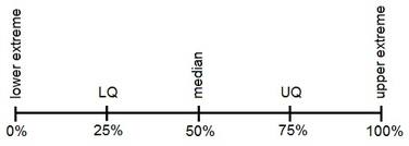
Percentiles and Quartiles
The mean and median are special cases of a family of parameters known as location parameters. These descriptive measures are called location parameters because they can be used to designate certain positions on the horizontal axis when the distribution of a variable is graphed.
Percentile:
- Percentiles are numerical values that divide an ordered data set into 100 groups of values with at the most 1% of the data values in each group. There can be maximum 99 percentile in a data set.
- A percentile is a measure that tells us what percent of the total frequency scored at or below that measure.
Percentiles corresponding to a given data value: The percentile in a set corresponding to a specific data value is obtained by using the following formula
Number of values below X + 0.5
Percentile = ——————————————–
Number of total values in data set
Example: Calculate percentile for value 12 from the following data
13 11 10 13 11 10 8 12 9 9 8 9
Solution:
Step # 01: Arrange data values in ascending order from smallest to largest
| S. No |
1 |
2 |
3 |
4 |
5 |
6 |
7 |
8 |
9 |
10 |
11 |
12 |
| Observations or values |
8 |
8 |
9 |
9 |
9 |
10 |
10 |
11 |
11 |
12 |
13 |
13 |
Step # 02: The number of values below 12 is 9 and total number in the data set is 12
Step # 03: Use percentile formula
9 + 0.5
Percentile for 12 = ——— x 100 = 79.17%
12
It means the value of 12 corresponds to 79th percentile
Example2: Find out 25th percentile for the following data
6 12 18 12 13 8 13 11
10 16 13 11 10 10 2 14
SOLUTION
Step # 01: Arrange data values in ascending order from smallest to largest
| S. No |
1 |
2 |
3 |
4 |
5 |
6 |
7 |
8 |
9 |
10 |
11 |
12 |
13 |
14 |
15 |
16 |
| Observations or values |
2 |
6 |
8 |
10 |
10 |
10 |
11 |
11 |
12 |
12 |
13 |
13 |
13 |
14 |
16 |
18 |
Step # 2 Calculate the position of percentile (n x k/ 100). Here n = No: of observation = 16 and k (percentile) = 25
16 x 25 16 x 1
Therefore Percentile = ———- = ——— = 4
100 4
Therefore, 25th percentile will be the average of values located at the 4th and 5th position in the ordered set. Here values for 4th and 5th correspond to the value of 10 each.
(10 + 10)
Thus, P25 (=Pk) = ————– = 10
2
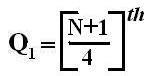
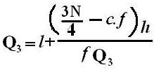
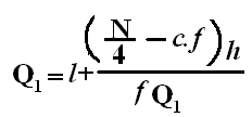
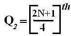
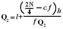
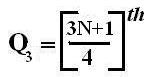
Quartiles
These are measures of position which divide the data into four equal parts when the data is arranged in ascending or descending order. The quartiles are denoted by Q.
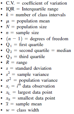
Symbol Key:

 Mean Deviation:
 Formula
OR S2 =
Calculating variance: Heart rate of certain patient is 80, 84, 80, 72, 76, 88, 84, 80, 78, & 78. Calculate variance for this data.
Solution:
Step 1:
Find mean of this data
Formula
OR S2 =
Calculating variance: Heart rate of certain patient is 80, 84, 80, 72, 76, 88, 84, 80, 78, & 78. Calculate variance for this data.
Solution:
Step 1:
Find mean of this data
 Variance = 184/ 10-1 = 184/9
Variance = 20.44
Standard Deviation
Variance = 184/ 10-1 = 184/9
Variance = 20.44
Standard Deviation
 Formula:
OR S =
Calculating Standard Deviation (we use same example): Heart rate of certain patient is 80, 84, 80, 72, 76, 88, 84, 80, 78, & 78. Calculate standard deviation for this data.
SOLUTION:
Step 1: Find mean of this data
Formula:
OR S =
Calculating Standard Deviation (we use same example): Heart rate of certain patient is 80, 84, 80, 72, 76, 88, 84, 80, 78, & 78. Calculate standard deviation for this data.
SOLUTION:
Step 1: Find mean of this data
 MERITS AND DEMERITS OF STD. DEVIATION
 is close to zero.


 Symbol Key: